Let's look at a toy example to understand how the two functions SUMIF() and VLOOKUP() can be used. Let's say you run a liquor shop and you need to keep track of the number of drinks you sell, and their price where each drink has a different price.
We are going to use VLOOKUP to lookup the price of a drink. Similarly, we are going to use SUMIF to calculate the total cost of individual drinks.
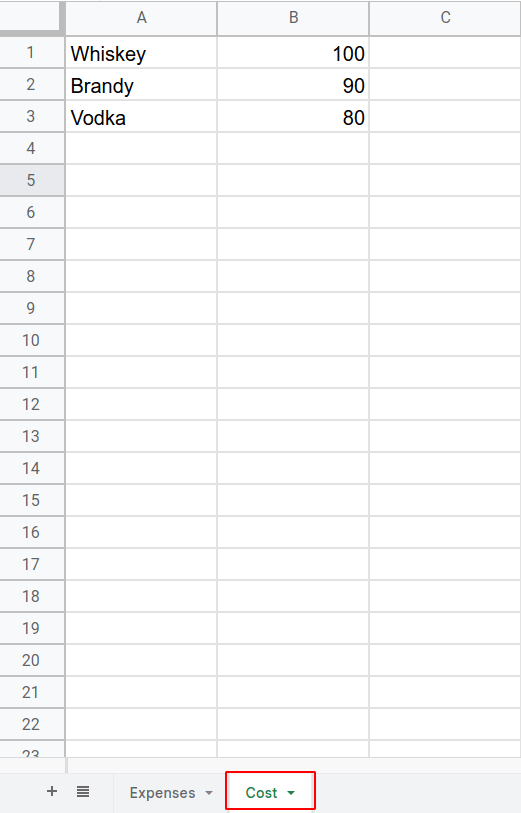
The lookup table looks like this. (Note the lookup table is in a different sheet)
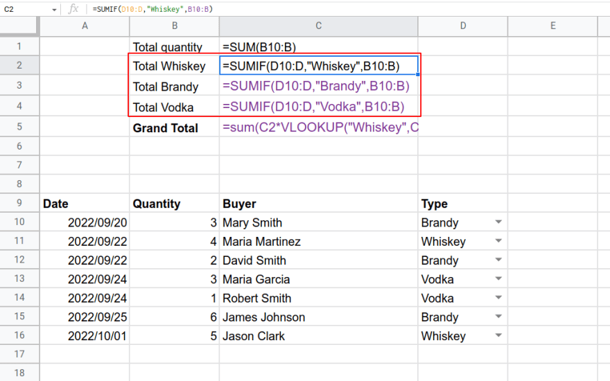
Now let's look at the expenses sheet.
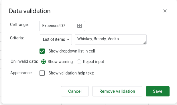
I added a dropdown in the type of liquor column with the three types of liquor:
Next, let's look at how we are using SUMIF.
SUMIF checks the string passed in the second argument against the value of the cell referenced by first argument, and if it matches, returns the value of the cell specified in the third argument. More info 1, 2
Let's look at how we are using VLOOKUP.
The first argument is the string we are searching for, the second argument specifies the range of cells to search for the first argument, the third argument specifies which column to return from the result and the fourth argument returns an exact match. More info 1, 2.
Click here for the complete example.


Top comments (0)