Monitoring the Yezin Dam: A Journey Through Time with Computer Vision

Introduction

Nestled near Yezin village, east of the Yangon-Mandalay Highway, lies the Yezin Dam — an essential infrastructure contributing to the agricultural prosperity of Zayarthiri Township in Nay Pyi Taw City, Myanmar. Constructed in 1975, the dam’s primary purpose is to facilitate irrigation for the surrounding agricultural areas and mitigate flooding from Sinthay and Yezin Streams.

Motivation for Monitoring: The Yezin Dam stands as a testament to human-engineered solutions addressing crucial water resource challenges. The motivation behind monitoring this vital structure over time is deeply rooted in understanding its dynamic interactions with the environment. By tracking changes in water levels, we aim to unravel insights into climate influences, dam management practices, and the broader implications for the region’s water resources.

Google Timelapse: A Window to the Past

To embark on this temporal exploration, we turn to Google Timelapse — a powerful tool harnessing the extensive satellite imagery archive from 1984 to 2022. This remarkable resource allows us to observe the evolution of landscapes, including the Yezin Dam, with unprecedented clarity. The time-lapse imagery offers a unique perspective, enabling the observation of long-term trends and environmental transformations.

By leveraging Google Timelapse, we gain access to a visual chronicle of the Yezin Dam’s journey through decades. This comprehensive dataset serves as the foundation for our endeavor to employ advanced computer vision techniques, providing a nuanced understanding of how the dam and its surroundings have changed over time.

Timelapse – Google Earth Engine

Explore the dynamics of our changing planet over the past three and a half decades.

earthengine.google.com

Data Collection Insights

Google Timelapse Unveiled

Our exploration of the Yezin Dam’s temporal evolution commenced with the bountiful imagery from Google Timelapse, spanning 1984 to 2022. This visual journey provided a captivating narrative of the dam’s transformation over nearly four decades.

Here are some sample satellite images from Google Timelapse of Yezin Dam for certain years(1996–2002):

Crafting Uniformity Amidst Diversity

Navigating the terrain of data collection, we confronted a formidable challenge — divergent resolutions and sizes spanning different years. Achieving analytical consistency necessitated a dedicated effort to standardize these images. The intricate yet pivotal task of harmonizing disparate shapes and sizes became our focus, demanding precision to ensure uniformity across the dataset.

Amidst this endeavor, we encountered additional challenges. The unyielding nature of the images restricted any alteration to their resolution or dimensions. Attempts to upscale the images proved counterproductive, yielding unexpected and random results. Moreover, experimenting with upscaling and subsequent model application resulted in outcomes contrary to our expectations, adding another layer of complexity to the data processing journey. Despite these hurdles, we persisted with resilience, employing online tools to meticulously transform the varied images into a cohesive and standardized collection.
Then we used some online tools to get the image set with equal dimensions and sizes.

Model Selection: UNET Water Body Segmentation

gauthamk02 / pytorch-waterbody-segmentation

PyTorch implementation of image segmentation for identifying water bodies from satellite images

title	emoji	colorFrom	colorTo	sdk	sdk_version	app_file	pinned
Water Body Segmentation	🤗	blue	gray	gradio	3.10.0	app.py	false

UNET Water Body Segmentation - PyTorch

This project contains the code for training and deploying a UNET model for water body segmentation from satellite images. The model is trained on the Satellite Images of Water Bodies from Kaggle. The model is trained using PyTorch and deployed using Gradio on Hugging Face Spaces.

🚀 Getting Started

All the code for training the model and exporting to ONNX format is present in the notebook folder or you can use this Kaggle Notebook for training the model. The app.py file contains the code for deploying the model using Gradio.

🤗 Demo

You can try out the model on Hugging Face Spaces

🖥️ Sample Inference

View on GitHub

Our model of choice, UNET Water Body Segmentation, stands as a testament to precision in the realm of semantic segmentation. Trained on Kaggle’s Satellite Images of Water Bodies, it emerged from Hugging Face’s repository, showcasing a prowess that aligns seamlessly with our project’s core objectives.

Why UNET?

In our pursuit of understanding water body dynamics over time, UNET’s reputation for accurate semantic segmentation made it the perfect ally. Its knack for unraveling intricate details in images aligns precisely with our mission to decode the evolving story of Yezin Dam.

Kaggle’s Tapestry, ONNX’s Canvas

Transitioning from Kaggle’s rich dataset to a model in the ONNX format, we ensured a smooth integration of the UNET model into our computational journey. This model, with its Kaggle-honed accuracy, becomes not just a tool but a guiding compass in our exploration of Yezin Dam’s aquatic chronicle.

Implementation

import cv2
import numpy as np
import onnxruntime as rt
import matplotlib.pyplot as plt
import os

# Assuming your images are in a folder named 'image-set'
images_folder = '../image-set'
onnx_path = '../weights/model.onnx'

# Get a list of all image files in the folder
image_files = [f for f in os.listdir(images_folder) if f.endswith('.png')]

# Load the ONNX model
session = rt.InferenceSession(onnx_path)
input_name = session.get_inputs()[0].name
output_name = session.get_outputs()[0].name

# Lists to store data for plotting
years = []
waterbody_areas = []

for img_file in image_files:
    # Extract the year from the image file name (assuming the file name has the format 'YYYY.png')
    year = int(img_file[:4])

    # Construct the full path to the image
    img_path = os.path.join(images_folder, img_file)

    # Read and preprocess the image
    orig_image = cv2.imread(img_path)
    orig_dim = orig_image.shape[:2]
    orig_image = cv2.cvtColor(orig_image, cv2.COLOR_BGR2RGB)

    image = np.array(orig_image, dtype=np.float32) / 255.0
    image = cv2.resize(image, (256, 256))
    image = np.transpose(image, (2, 0, 1))
    image = np.expand_dims(image, axis=0)

    # Perform inference
    pred_onx = session.run([output_name], {input_name: image.astype(np.float32)})[0]
    pred_onx = pred_onx > 0.5
    pred_onx = cv2.resize(pred_onx[0, 0].astype(np.uint8), (orig_dim[1], orig_dim[0]))

    # Calculate and store waterbody area for each image
    waterbody_area = np.count_nonzero(pred_onx)
    years.append(year)
    waterbody_areas.append(waterbody_area)

    # Display the results (you can modify this part as needed)
    plt.figure(figsize=(10, 10))
    plt.subplot(1, 2, 1)
    plt.imshow(orig_image)
    plt.title('Original Image')
    plt.subplot(1, 2, 2)
    plt.imshow(pred_onx, cmap='gray')
    plt.title('Predicted Mask')
    plt.show()

# Plotting the waterbody areas over time
plt.figure(figsize=(10, 6))
plt.plot(years, waterbody_areas, marker='o')
plt.title('Waterbody Areas Over Time')
plt.xlabel('Year')
plt.ylabel('Waterbody Area')
plt.grid(True)
plt.show()

Results of Code Implementation and Analysis

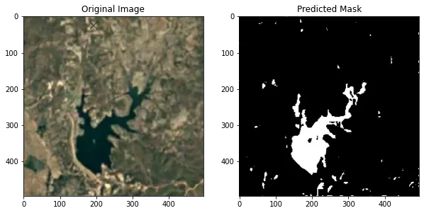
Here are some images showing the original satellite image imported from Google Timelapse of Yezin Dam and the predicted masked image of the corresponding year:

Waterbody area in 1984

Waterbody area in 1989

Waterbody area in 1993

Waterbody area in 1999

Waterbody area in 2006

Waterbody area in 2011

Waterbody area in 2015

Waterbody area in 2019

Waterbody area in 2022

Here is the Plot of Yezin Dam water body areas Over the time from 1984 to 2022:

Early 1990s Surge (1993):

• Observation: Substantial increase in waterbody area, reaching a peak in 1993 (57,633 square units). Possible Reasons:
• Increased rainfall during this period could have contributed to higher water levels.
• Changes in dam management practices or water release policies may have played a role.

1999 Drop:

• Observation: Significant drop in waterbody area in 1999 (19,064 square units). Possible Reasons:
• Reduced rainfall or changes in weather patterns might have led to a decrease in water levels.
• Increased water usage, possibly for irrigation or other purposes.

2006 Surge:

• Observation: Remarkable surge in waterbody area in 2006 (62,339 square units). Possible Reasons:
• Heavy rainfall during this period could have caused an increase in water levels.
• Dam-related activities, such as reservoir management or construction, might have influenced the waterbody area.

2011 and 2019 Peaks:

• Observation: Elevated waterbody areas in 2011 and 2019. Possible Reasons:
• Climate events such as increased rainfall or variations in precipitation patterns.
• Changes in dam operation or water management practices during these years.

Recent Stability (2015–2022):

• Observation: More stable waterbody areas in recent years (2015–2022). Possible Reasons:
• Improved water management practices or reservoir control measures.
• Climate conditions leading to consistent water levels.

Insights from Research Paper

We got to find a research paper on Water level changes in Yezin dam that was published in Scientific Research Journal (SCIRJ), Volume VII, Issue VIII, August 2019.

drive.google.com

As the Water level of the dam is proportional to its area, we are considering this paper to review and get some insights.

Climate Conditions:

• The study area experiences a Tropical Savanna Climate (AW) according to the Köppen Climate Classification. The average temperature increased slightly from 26.97°C in 2006 to 28.14°C in 2016. However, this change alone may not be a dominant factor in water surface area variation.

• Rainfall plays a crucial role. The total average rainfall for the 10 years was 1279.93 cm, with fluctuations in individual years (139.47 cm in 2006, 152.09 cm in 2011, and 137.39 cm in 2016). Changes in rainfall patterns could significantly impact water levels.

Inflow and Outflow Data:

• The study includes data on total inflow and outflow from the dam. In 2006, inflow was 48,716 m³, and outflow was 46,391 m³. In 2011, inflow increased to 58,473 m³, and outflow decreased to 36,683 m³. By 2016, both inflow and outflow significantly reduced to 19,938 m³ and 4,778 m³, respectively.
• The decrease in outflow may indicate increased water retention or reduced water release, affecting the overall water surface area.

Normalized Difference Water Index (NDWI):

• The research employed NDWI using Landsat satellite images to assess water surface changes. NDWI is calculated based on the normalized relationship between the green and near-infrared portions of the spectrum. A decrease in NDWI values could indicate a reduction in water surface area.

Accuracy Assessment:

• The study assessed the accuracy of its methods, reporting an accuracy of 97% in 2006, 79.15% in 2011, and 92.2% in 2016. Discrepancies in accuracy may be attributed to factors like spatial resolution, ground data quality, or image processing techniques.

Technical Limitations:

• The research acknowledges limitations such as the failure of the Scan Line Corrector (SLC) in Landsat 7, leading to data gaps. Techniques like gap-filling were employed to address this issue.

Water Management Practices:

• Human interventions such as the construction of drainage channels, water supply for rural and urban areas, and irrigation for agriculture could contribute to changes in water surface area.

Land Use Dynamics:

• The combined use of Remote Sensing (RS) and Geographic Information System (GIS) helps detect land use dynamics. Changes in the surrounding land cover might impact water flow and storage.

Conclusion

Embarking on the implementation journey, the essence of my vision algorithm’s success lies in meticulous data preprocessing and model selection. Rigorous steps were taken to curate a robust dataset, with careful consideration given to image quality and relevance. The adoption of the UNET Water Body Segmentation model from Hugging Face Space aligns seamlessly with the project’s objectives, leveraging its proficiency in analyzing satellite images of water bodies. The utilization of the ONNX format facilitates seamless integration into the workflow, ensuring efficient model deployment. The code implementation involves a systematic approach, from loading the model to processing images, conducting inference, and generating masked images highlighting water body areas. The emphasis on visualizing results at each step not only aids in debugging but also enhances interpretability. The subsequent analysis of water body areas over time provides valuable insights into the dynamic changes around the Yezin Dam, aligning with the overarching goal of understanding and monitoring the evolution of water bodies.