Machine Learning is an innovative and important field in the industry. The type of algorithm we choose for our ML program changes depending on what we want to accomplish.
There are quite a few algorithms out there, so it can be pretty overwhelming for beginners. Today, we will briefly introduce the 10 most popular learning algorithms so you can get comfortable with the exciting world of Machine Learning!
Let’s jump right in!
Want to get right to learning with hands-on practice? Check out Educative’s course, Grokking Data Science.
1. Linear Regression
Linear Regression is likely the most popular ML algorithm. Linear regression finds a line that best fits a scattered data points on a graph. It attempts to represent the relationship between independent variables (the x values) and a numeric outcome (the y values) by fitting the equation of a line to that data. This line can then be used to predict values to come!
The most popular technique for this algorithm is least of squares. This method calculates the best-fitting line such that the vertical distances from each data point of the line are minimum. The overall distance is the sum of the squares of the vertical distances (green lines) for all the data points. The idea is to fit a model by minimizing this squared error or distance.
2. Logistic Regression
Logistic regression is similar to linear regression, but it is used when the output is binary (i.e. when outcome can have only two possible values). The prediction for this final output will be a non-linear S-shaped function called the logistic function, g().
This logistic function maps the intermediate outcome values into an outcome variable Y with values ranging from 0 to 1. These values can then be interpreted as the probability of occurrence of Y. The properties of the S-shaped logistic function make logistic regression better for classification tasks.
3. Decision Trees
Decision Trees can be used for both regression and classification tasks.
In this algorithm, the training model learns to predict values of the target variable by learning decision rules with a tree representation. A tree is made up of nodes with corresponding attributes.
At each node we ask a question about the data based on the available features. The left and right branches represent the possible answers. The final nodes, leaf nodes, correspond to a predicted value.
The importance for each feature is determined in a top-down approach. The higher the node, the more important its attribute.
An example decision tree that decides whether or not to wait at a restaurant:
4. Naive Bayes
Naive Bayes is based on the Bayes Theorem. It measures the probability of each class, and the conditional probability for each class give values of x. This algorithm is used for classification problems to reach a binary yes/no outcome. Take a look at the equation below.
- P(c|x) = probability of the event of class c, given the predictor variable x,
- P(x|c) = probability of x given c,
- P( c) = probability of the class,
- P(x) = probability of the predictor.
Naive Bayes classifiers are a popular statistical technique for filtering spam emails!
5. Support Vector Machines (SVM)
SVM is a supervised algorithm used for classification problems. SVM tries to draw two lines between the data points with the largest margin between them. To do this, we plot data items as points in n-dimensional space, where n is the number of input features. Based on this, SVM finds an optimal boundary, called a hyperplane, which best separates the possible outputs by their class label.
The distance between the hyperplane and the closest class point is called the margin. The optimal hyperplane has the largest margin that classifies points to maximize the distance between the closest data point and both classes.
6. K-Nearest Neighbors (KNN)
KNN algorithm is very simple. KNN classifies an object by searching through the entire training set for the k most similar instances, the k neighbors, and assigning a common output variable to all those k instances.
The selection of k is critical: a small value can result in a lot of noise and inaccurate results, while a large value is not feasible. It is most commonly used for classification, but it is also useful for regression problems.
The distance functions for assessing similarity between instances can be Euclidean, Manhattan, or Minkowski distance. Euclidean distance is an ordinary straight-line distance between two points. It is actually the square root of the sum of the squares of the differences between the coordinates of the points.
7. K-Means
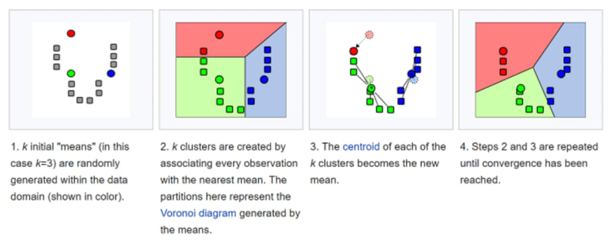
K-means is to cluster by classify data sets. For example, this algorithm could be used to segment users into groups based on purchase history. It finds K number of clusters in the dataset. K-Means is for unsupervised learning, so we only use training data, X, and the number of clusters, K, that we want to identify.
The algorithm iteratively assigns each data point to one of the K groups based on their features. It picks k points for each of the K-clusters, known as the centroid. A new data point is added to the cluster with the closest centroid based on similarity. This process continues until the centroids stop changing.
8. Random Forest
Random Forest is a very popular ensemble ML algorithm. The underlying idea for this algorithm is that the opinion of many is more accurate than the individual. In Random Forest, we use an ensemble of decision trees (see #3).
To classify a new object, we take a kind of vote from each decision tree, combine the outcome, and make a final decision based on majority vote.
(a) In the training process, each decision tree is built based on a bootstrap sample of the training set. (b) In the classification process, decision for the input instance is based on the majority vote.
9. Dimensionality Reduction
Due to the sheer amount of data we can capture today, machine learning problems have become more complicated. This means that training is extremely slow, and it’s harder to find a good solution. This problem is often called the curse of dimensionality.
Dimensionality reduction attempts to solve this problem by assembling specific features into higher-level ones without losing the most important information. Principal Component Analysis (PCA) is the most popular dimensionality reduction technique.
PCA reduces the dimension of a dataset by squashing it onto a lower-dimensional line, or a hyperplane/subspace. This retains as much of the original data’s salient characteristics as possible.
10. Artificial Neural Networks (ANN)
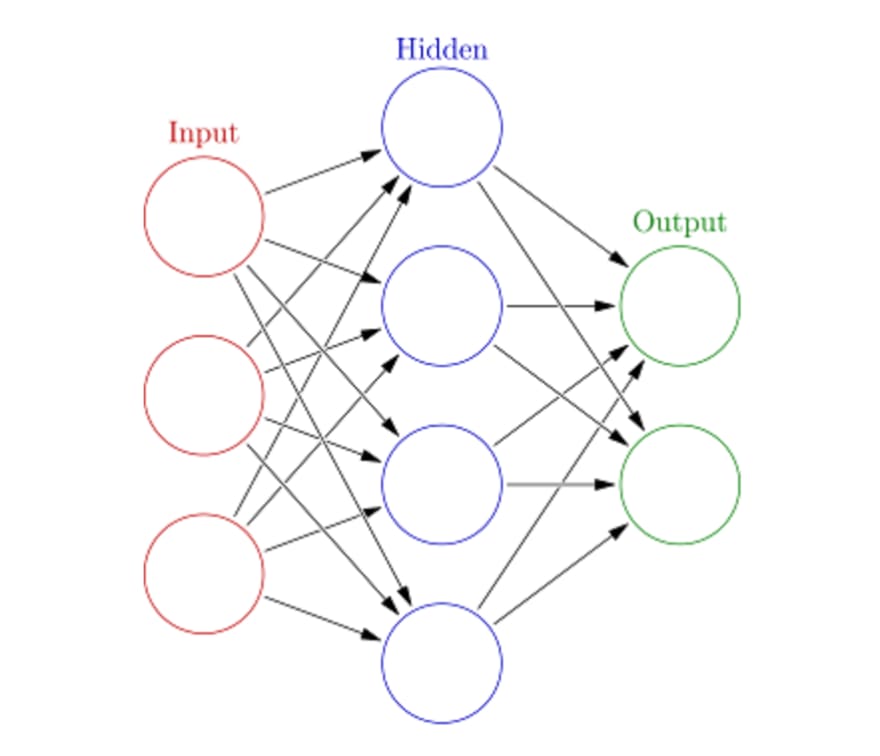
ANN can handle large, complex ML tasks. A neural network is essentially a set of interconnected layers with weighted edges and nodes called neurons. Between the input and output layers we can insert multiple hidden layers. ANN uses two hidden layers. Beyond that, we are dealing with Deep Learning.
ANN works similar to the brain’s architecture. A set of neurons are assigned a random weight that determine how neurons process input data. The relationship between inputs and outputs is learned by training the neural network on input data. During the training phase, the system has access to the correct answers.
If the network doesn’t accurately identify the input, the system adjusts the weights. After sufficient training, it will consistently recognize the correct patterns.
Each circular node represents an artificial neuron and an arrow represents a connection from the output of one artificial neuron to the input of another.
Conclusion
Now you have foundational introduction to the most popular machine learning algorithms. You’re ready to move onto more complicated concepts, or even implement them with deep-dive, hands-on practice. If you want to see how to implement these algorithms, check out Educative’s Grokking Data Science course, which applies these exciting theories in clear, real-world applications.
Start your Machine Learning journey today!
Happy learning!


Top comments (0)